Beveridge-Nelson Filter United States • bnfilter

This example uses the updated US GDP dataset through to 2023 Q2.

library(bnfilter)
head(usgdp)
#>          Qtr1     Qtr2     Qtr3     Qtr4
#> 1947 2182.681 2176.892 2172.432 2206.452
#> 1948 2239.682 2276.690

Take the log(usgdp) * 100.0

y <- transform_series(y=usgdp, take_log=TRUE, pcode = "p1")

Example with dynamic demean

bnfOutput <- bnf(y=y,
  delta_select = 2,
  demean = "dm",
  iterative = 100,
  dynamic_bands = TRUE,
  adjusted_bands = TRUE,
  outliers = c(293, 294),
  window = 40,
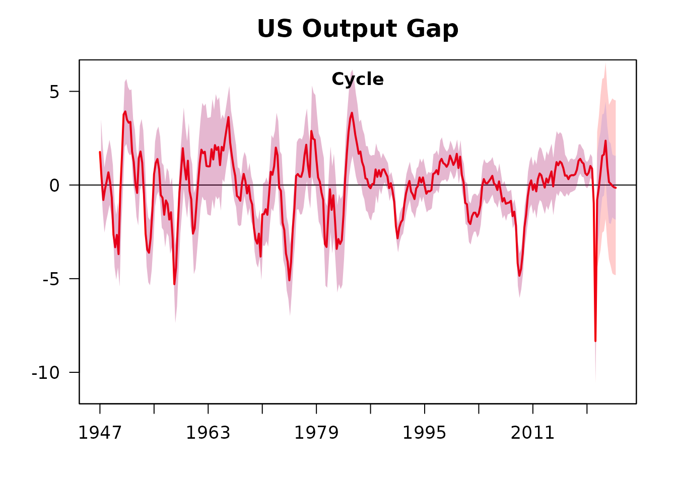
  ib = TRUE)

United States Output Gap, with adjusted bands and outlier adjustment for COVID19:

plot(bnfOutput, main = "US Output Gap")
#> Warning in matrix(data = c(1, 2), nrow = 1, ncol = 1): data length differs from
#> size of matrix: [2 != 1 x 1]